Sample Module

Calculating Spend

Description

Calculating spend is daily task if you work in apparel sourcing or buying.
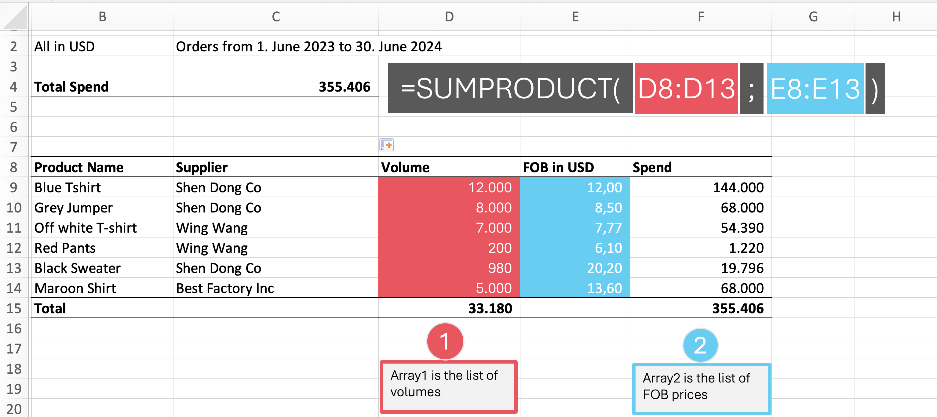
In this example we go through how to present spend values in a table and also introduce the function SUMPRODUCT.

Let's take a look:

This function is useful to calculate the total spend of products with suppliers.
For example, you have the FOB (Free on Board) price and the volume of products you purchased from various suppliers.
We will be creating a table which shows volumes of products by supplier, here is the video:

Video Calculating Spend:

Let's dive a bit deeper and assume that have the supplier spend this year and the supplier spend of last year and want to compare the two.

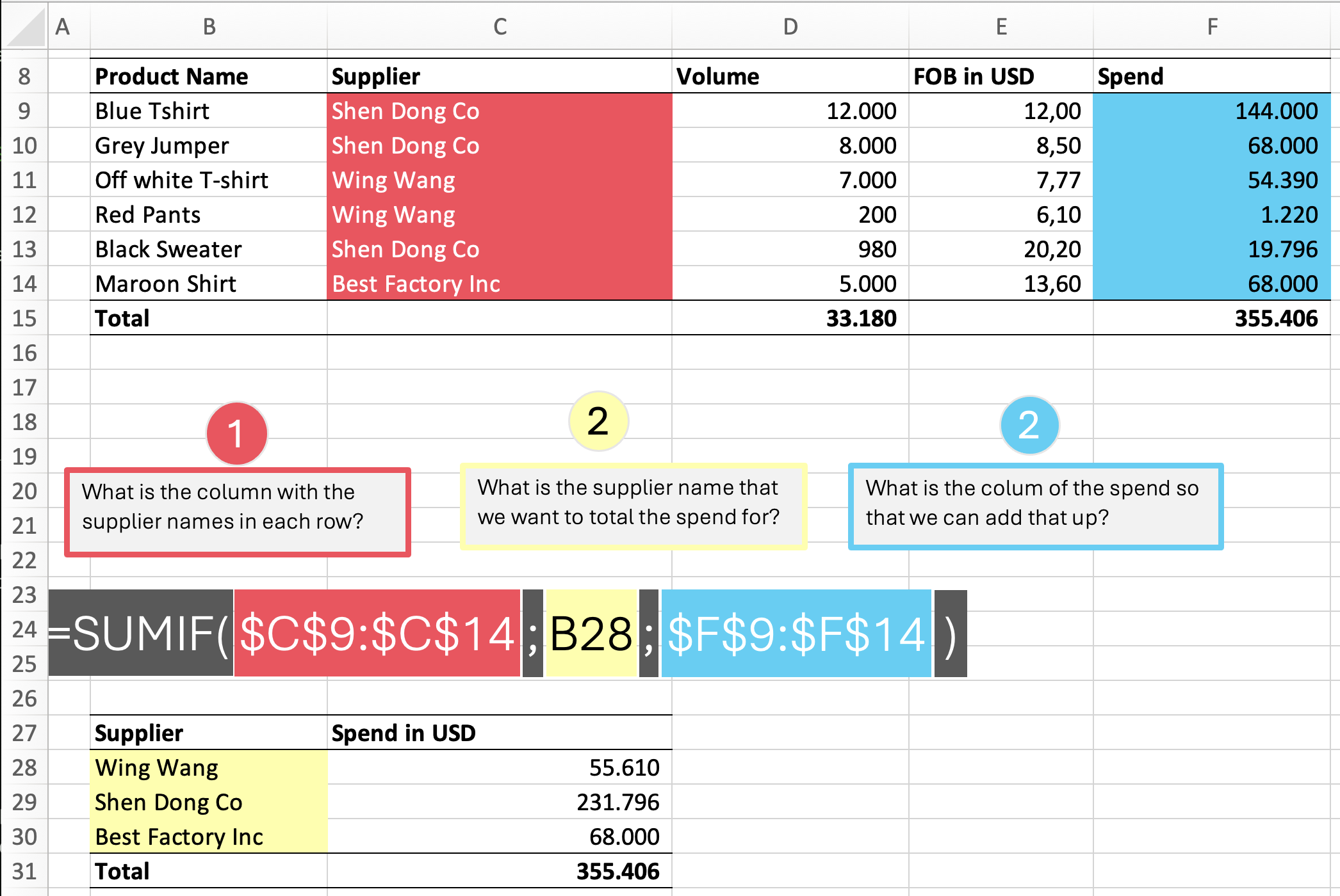
An important concept in Excel is to fix the cells you are referring to. In the above SUMIF example, we fix the range and the sum range. The range being the supplier column (C9:C14) and the sum range the spend (F9:F14). Instead of writing the formula every time, we want to copy it down from cell C28 to C30. If we would copy the formula without the cells fixed (no $ sign before the column and row) then the range would change.

In the course we have a specific module on fixing cells to this as it's one of the most important concepts of Excel.

This is a sample module so you know more what you will get when you sign up to the course but it's a real module and we hope you found it useful. Any comments or questions just email us course@apparelofcourse.com. Thanks